A Visual Exploration of Neural Radiance Fields

Generating new views of a scene from limited input images — novel view synthesis — is hard. Traditional methods force a choice between flexibility and realism. Neural Radiance Fields (NeRF) learn a scene’s 3D structure and appearance directly from sparse 2D images, enabling photorealistic view synthesis. This post explains how NeRFs work and the trade-offs involved.

Volume Rendering

First, some background on 3D object representation. A “volume” spans three spatial dimensions, denoted $V : \mathbb{R}^3 \rightarrow F$, with “features” for each point in space (density, texture). Unlike meshes, defined solely by surface structure, volumes capture both surface and interior. This makes volumes natural for semi-transparent objects: clouds, smoke, liquids. For our purposes, the interesting features are color $RGB$ and density $\sigma$.

Rendering a 2D image from a volume means computing “radiance” — the reflection, refraction, and emittance of light from object to observer — to generate an $RGB$ pixel grid.

NeRF uses Ray Marching for volume rendering. Ray Marching constructs rays $\mathbf{r}(t) = \mathbf{o} + t\mathbf{d}$ with origin and direction vectors for each pixel. Sampling along each ray yields color $c_i$ and density $\sigma_i$.

A transfer function (from classical volume rendering ¹) forms an RGBA sample by accumulating from the point closest to the eye to the volume exit. Discrete form:

where $T_i = \prod^{i-1}_{j=1} (1 - \alpha_j)$, $\alpha_i = 1 - e^{-\sigma_i \delta_i}$, and $\delta_i$ is the sampling distance.

The transfer function captures an intuitive idea: objects behind dense or opaque materials contribute less to the final image than those behind transparent materials. Flowers behind a glass vase are more visible than flowers behind an opaque ceramic vase.

The rendering component must be differentiable for gradient descent optimization ². This allows fine-tuning based on the gap between rendered and target images.

The true innovation lies not in rendering, but in encoding the volume. NeRF addresses two challenges:

1. How can we encode the volume to query any arbitrary point in space? This enables rendering from viewpoints not in the original dataset.

2. How can we account for non-matte surfaces? Matte surfaces scatter light uniformly, but glossy and specular materials have complex reflectance. A NeRF trained on a shiny metal sculpture should capture its specular highlights and reflections.

While differentiable rendering enables optimization, NeRF’s innovation lies in encoding: query-ability at arbitrary points and handling non-matte surfaces.

Volume Representation

Consider a naive approach: voxel grids. Voxel grids discretize 3D space into cubes, storing metadata in an array (material, color, viewpoint-specific features). The challenge: no advantage from natural symmetries, and storage/rendering requirements explode in $O(N^3)$. Viewpoint-specific reflections and lighting need separate handling in rendering.

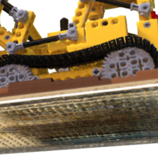
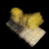
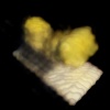
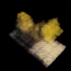
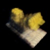
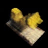
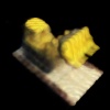
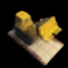
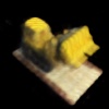
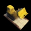
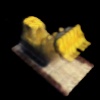
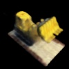
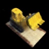
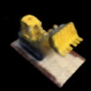
You can get a good feel for the performance impact by increasing the level of granularity in the Sine-wave Voxel Grid. I encourage you to compare this level of detail and fluidity to our NeRF Lego bulldozer.

Neural Radiance Fields (NeRF)

What is a volume if not a function mapping? Volumes have symmetries we’d like to exploit. Densely connected neural networks with ReLU activations ³ are excellent approximators given sufficient data.

NeRF ⁴ uses densely connected ReLU networks (8 layers of 256 units) to represent volume. The network $F_\theta$ outputs $RGB\sigma$ for each spatial/viewpoint pair. This implicitly encodes material properties — lighting, reflectance, transparency — normally specified manually. NeRF learns a continuous, high-fidelity scene representation from input images:

Optimizing

To optimize NeRF, a volume renderer generates a 2D image from the learned 3D representation by ray marching and accumulating color/density values. Comparing this to ground truth yields a pixel-squared error loss. Minimizing this loss via gradient descent teaches the model to represent the scene accurately.

NeRF works for novel view synthesis ⁴, dynamic scenes ⁵, and large-scale reconstruction ⁶. Learning high-fidelity, continuous representations from input images makes it powerful for computer vision and graphics.

Challenges

Where can NERF go wrong?

Despite the fantastic results, NERF is not a cure-all. It fails in very predictable ways.

Select region for more information.

Data Requirements and Training Times

A key challenge: NeRFs need substantial training data. Basic NeRF models have no prior knowledge — each model trains from scratch for each scene.

Data requirements vary with scene complexity and desired quality. A simple uniformly textured object needs fewer training images than a complex outdoor scene with intricate details and varying lighting.

Training a high-quality NeRF takes hours or days, depending on dataset size and compute. The original paper ⁴ reported 1-2 days for 100-400 images on a single GPU. These training times limit practical applications, especially for large-scale or dynamic scenes.

We can see the impact that has on both training time, and the data requirements in our training simulator.

Iteration: 300

Real Time: 491s

A "tiny" NeRF trained on 100 viewpoints of our bulldozer randomly sampled in batches of 64 per iteration. Notably, we use a ReLU model with 9 densely connected layers of 256 outputs with the viewpoint concatenated halfway through the model architecture.

Special Sauce

The above examples lack the clarity of published NeRFs. Beyond training time, state-of-the-art performance requires a few additional techniques.

Held-out Viewing Directions

Leave viewing direction out of the first 4 layers. This reduces view-dependent (often floating) artifacts that occur when the model prematurely optimizes view-dependent features before learning spatial structure.

Fourier Transforms

The original NeRF doesn’t use raw RGB images and viewpoints as input — it transforms them using Fourier features. Fourier transforms decompose signals into constituent frequencies. Applying Fourier features to input coordinates lets the network capture high-frequency details essential for fine structures and textures.

The precise mechanism to utilise Fourier features is to apply a pre-processing step to transform the position into sinusoidal signals of exponential frequencies.

Densely connected ReLU networks cannot model signals with fine detail or represent spatial/temporal derivatives essential to physical signals. Sitzmann ⁷ reached a similar realization, though they changed the activation function rather than pre-processing inputs.

Imagine a simple 1D signal with sharp edges and fine details. A standard ReLU MLP would struggle, producing smoothed or blurred output. Fourier feature transformation lets the network capture high-frequency components, representing sharp edges and fine details accurately.

This seemingly arbitrary trick yields substantially better results and removes the tendency to blur images, letting the network capture essential spatial and temporal derivatives.

Comparison of Fourier Features vs Raw Position

Fourier Features allow for high frequency functions in low domains.

Set the visibility of one image over the other. 0 is full visibility of the second image and 100 is full visibility of the first image. Any amount in-between is a left/right cutoff at the percentage of the slider.

Iteration 250

Set the visibility of one image over the other. 0 is full visibility of the second image and 100 is full visibility of the first image. Any amount in-between is a left/right cutoff at the percentage of the slider.

Iteration 500

Set the visibility of one image over the other. 0 is full visibility of the second image and 100 is full visibility of the first image. Any amount in-between is a left/right cutoff at the percentage of the slider.

Iteration 750

Set the visibility of one image over the other. 0 is full visibility of the second image and 100 is full visibility of the first image. Any amount in-between is a left/right cutoff at the percentage of the slider.

Iteration 1000

The stationary property of Fourier feature dot products (Positional Encoding is one type) is essential. Stationarity means statistical properties remain constant across positions. The similarity between two points in transformed space depends only on their relative positions, not absolute locations.

Stationarity lets the ReLU MLP learn weights that capture high-frequency components regardless of position. These learned weights correspond to periodic functions. These functions represent the transformed signal’s high-frequency components.

Hierarchical Sampling

An obvious question about classical volume rendering: why use uniform sampling when most models have large empty spaces (low densities) and diminishing value from samples behind dense objects?

The original NeRF ⁴ learns two models: a coarse-grained model for density estimates and a fine-grained model identical to the original. The coarse model re-weights fine-grained sampling, producing better results.

Conclusion

You now have an overview of Neural Radiance Fields and how they work. NeRFs offer a flexible, powerful framework for encoding and rendering 3D scenes. The original approach has limitations — substantial data requirements and long training times — but ongoing research addresses these challenges and expands NeRF capabilities. As the field evolves, expect advancements making NeRFs more practical and accessible.